In this tutorial, we will answer some common questions about autoencoders, and we will cover code examples of the following models:
- a simple autoencoder based on a fully-connected layer
- a sparse autoencoder
- a deep fully-connected autoencoder
- a deep convolutional autoencoder
- an image denoising model
- a sequence-to-sequence autoencoder
- a variational autoencoder
Note: all code examples have been updated to the Keras 2.0 API on March 14, 2017. You will need Keras version 2.0.0 or higher to run them.
What are autoencoders?
"Autoencoding" is a data compression algorithm where the compression and decompression functions are 1) data-specific, 2) lossy, and 3) learned automatically from examples rather than engineered by a human. Additionally, in almost all contexts where the term "autoencoder" is used, the compression and decompression functions are implemented with neural networks.
1) Autoencoders are data-specific, which means that they will only be able to compress data similar to what they have been trained on. This is different from, say, the MPEG-2 Audio Layer III (MP3) compression algorithm, which only holds assumptions about "sound" in general, but not about specific types of sounds. An autoencoder trained on pictures of faces would do a rather poor job of compressing pictures of trees, because the features it would learn would be face-specific.
2) Autoencoders are lossy, which means that the decompressed outputs will be degraded compared to the original inputs (similar to MP3 or JPEG compression). This differs from lossless arithmetic compression.
3) Autoencoders are learned automatically from data examples, which is a useful property: it means that it is easy to train specialized instances of the algorithm that will perform well on a specific type of input. It doesn't require any new engineering, just appropriate training data.
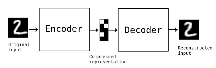
To build an autoencoder, you need three things: an encoding function, a decoding function, and a distance function between the amount of information loss between the compressed representation of your data and the decompressed representation (i.e. a "loss" function). The encoder and decoder will be chosen to be parametric functions (typically neural networks), and to be differentiable with respect to the distance function, so the parameters of the encoding/decoding functions can be optimize to minimize the reconstruction loss, using Stochastic Gradient Descent. It's simple! And you don't even need to understand any of these words to start using autoencoders in practice.
Are they good at data compression?
Usually, not really. In picture compression for instance, it is pretty difficult to train an autoencoder that does a better job than a basic algorithm like JPEG, and typically the only way it can be achieved is by restricting yourself to a very specific type of picture (e.g. one for which JPEG does not do a good job). The fact that autoencoders are data-specific makes them generally impractical for real-world data compression problems: you can only use them on data that is similar to what they were trained on, and making them more general thus requires lots of training data. But future advances might change this, who knows.
What are autoencoders good for?
They are rarely used in practical applications. In 2012 they briefly found an application in greedy layer-wise pretraining for deep convolutional neural networks [1], but this quickly fell out of fashion as we started realizing that better random weight initialization schemes were sufficient for training deep networks from scratch. In 2014, batch normalization [2] started allowing for even deeper networks, and from late 2015 we could train arbitrarily deep networks from scratch using residual learning [3].
Today two interesting practical applications of autoencoders are data denoising (which we feature later in this post), and dimensionality reduction for data visualization. With appropriate dimensionality and sparsity constraints, autoencoders can learn data projections that are more interesting than PCA or other basic techniques.
For 2D visualization specifically, t-SNE (pronounced "tee-snee") is probably the best algorithm around, but it typically requires relatively low-dimensional data. So a good strategy for visualizing similarity relationships in high-dimensional data is to start by using an autoencoder to compress your data into a low-dimensional space (e.g. 32-dimensional), then use t-SNE for mapping the compressed data to a 2D plane. Note that a nice parametric implementation of t-SNE in Keras was developed by Kyle McDonald and is available on Github. Otherwise scikit-learn also has a simple and practical implementation.
So what's the big deal with autoencoders?
Their main claim to fame comes from being featured in many introductory machine learning classes available online. As a result, a lot of newcomers to the field absolutely love autoencoders and can't get enough of them. This is the reason why this tutorial exists!
Otherwise, one reason why they have attracted so much research and attention is because they have long been thought to be a potential avenue for solving the problem of unsupervised learning, i.e. the learning of useful representations without the need for labels. Then again, autoencoders are not a true unsupervised learning technique (which would imply a different learning process altogether), they are a self-supervised technique, a specific instance of supervised learning where the targets are generated from the input data. In order to get self-supervised models to learn interesting features, you have to come up with an interesting synthetic target and loss function, and that's where problems arise: merely learning to reconstruct your input in minute detail might not be the right choice here. At this point there is significant evidence that focusing on the reconstruction of a picture at the pixel level, for instance, is not conductive to learning interesting, abstract features of the kind that label-supervized learning induces (where targets are fairly abstract concepts "invented" by humans such as "dog", "car"...). In fact, one may argue that the best features in this regard are those that are the worst at exact input reconstruction while achieving high performance on the main task that you are interested in (classification, localization, etc).
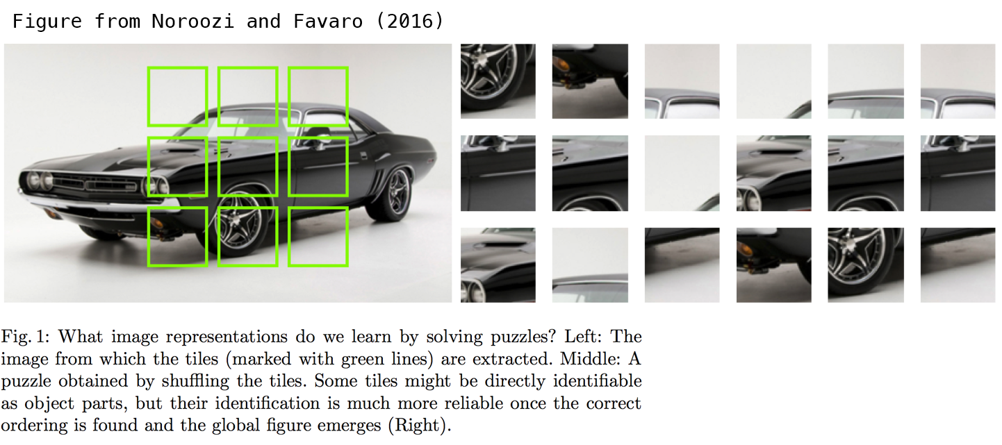
In self-supervized learning applied to vision, a potentially fruitful alternative to autoencoder-style input reconstruction is the use of toy tasks such as jigsaw puzzle solving, or detail-context matching (being able to match high-resolution but small patches of pictures with low-resolution versions of the pictures they are extracted from). The following paper investigates jigsaw puzzle solving and makes for a very interesting read: Noroozi and Favaro (2016) Unsupervised Learning of Visual Representations by Solving Jigsaw Puzzles. Such tasks are providing the model with built-in assumptions about the input data which are missing in traditional autoencoders, such as "visual macro-structure matters more than pixel-level details".
Let's build the simplest possible autoencoder
We'll start simple, with a single fully-connected neural layer as encoder and as decoder:
import keras
from keras import layers

# This is the size of our encoded representations
encoding_dim = 32  # 32 floats -> compression of factor 24.5, assuming the input is 784 floats

# This is our input image
input_img = keras.Input(shape=(784,))
# "encoded" is the encoded representation of the input
encoded = layers.Dense(encoding_dim, activation='relu')(input_img)
# "decoded" is the lossy reconstruction of the input
decoded = layers.Dense(784, activation='sigmoid')(encoded)

# This model maps an input to its reconstruction
autoencoder = keras.Model(input_img, decoded)
Let's also create a separate encoder model:
# This model maps an input to its encoded representation
encoder = keras.Model(input_img, encoded)
As well as the decoder model:
# This is our encoded (32-dimensional) input
encoded_input = keras.Input(shape=(encoding_dim,))
# Retrieve the last layer of the autoencoder model
decoder_layer = autoencoder.layers[-1]
# Create the decoder model
decoder = keras.Model(encoded_input, decoder_layer(encoded_input))
Now let's train our autoencoder to reconstruct MNIST digits.
First, we'll configure our model to use a per-pixel binary crossentropy loss, and the Adam optimizer:
autoencoder.compile(optimizer='adam', loss='binary_crossentropy')
Let's prepare our input data. We're using MNIST digits, and we're discarding the labels (since we're only interested in encoding/decoding the input images).
from keras.datasets import mnist
import numpy as np
(x_train, _), (x_test, _) = mnist.load_data()
We will normalize all values between 0 and 1 and we will flatten the 28x28 images into vectors of size 784.
x_train = x_train.astype('float32') / 255.
x_test = x_test.astype('float32') / 255.
x_train = x_train.reshape((len(x_train), np.prod(x_train.shape[1:])))
x_test = x_test.reshape((len(x_test), np.prod(x_test.shape[1:])))
print(x_train.shape)
print(x_test.shape)
Now let's train our autoencoder for 50 epochs:
autoencoder.fit(x_train, x_train,
                epochs=50,
                batch_size=256,
                shuffle=True,
                validation_data=(x_test, x_test))
After 50 epochs, the autoencoder seems to reach a stable train/validation loss value of about 0.09. We can try to visualize the reconstructed inputs and the encoded representations. We will use Matplotlib.
# Encode and decode some digits
# Note that we take them from the *test* set
encoded_imgs = encoder.predict(x_test)
decoded_imgs = decoder.predict(encoded_imgs)
# Use Matplotlib (don't ask)
import matplotlib.pyplot as plt

n = 10  # How many digits we will display
plt.figure(figsize=(20, 4))
for i in range(n):
    # Display original
    ax = plt.subplot(2, n, i + 1)
    plt.imshow(x_test[i].reshape(28, 28))
    plt.gray()
    ax.get_xaxis().set_visible(False)
    ax.get_yaxis().set_visible(False)

    # Display reconstruction
    ax = plt.subplot(2, n, i + 1 + n)
    plt.imshow(decoded_imgs[i].reshape(28, 28))
    plt.gray()
    ax.get_xaxis().set_visible(False)
    ax.get_yaxis().set_visible(False)
plt.show()
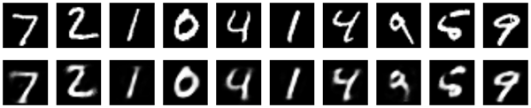
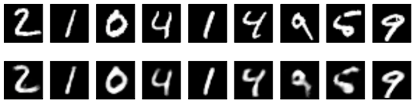
Here's what we get. The top row is the original digits, and the bottom row is the reconstructed digits. We are losing quite a bit of detail with this basic approach.
Adding a sparsity constraint on the encoded representations
In the previous example, the representations were only constrained by the size of the hidden layer (32). In such a situation, what typically happens is that the hidden layer is learning an approximation of PCA (principal component analysis). But another way to constrain the representations to be compact is to add a sparsity contraint on the activity of the hidden representations, so fewer units would "fire" at a given time. In Keras, this can be done by adding an activity_regularizer to our Dense layer:
from keras import regularizers

encoding_dim = 32

input_img = keras.Input(shape=(784,))
# Add a Dense layer with a L1 activity regularizer
encoded = layers.Dense(encoding_dim, activation='relu',
                activity_regularizer=regularizers.l1(10e-5))(input_img)
decoded = layers.Dense(784, activation='sigmoid')(encoded)

autoencoder = keras.Model(input_img, decoded)
Let's train this model for 100 epochs (with the added regularization the model is less likely to overfit and can be trained longer). The models ends with a train loss of 0.11 and test loss of 0.10. The difference between the two is mostly due to the regularization term being added to the loss during training (worth about 0.01).
Here's a visualization of our new results:
They look pretty similar to the previous model, the only significant difference being the sparsity of the encoded representations. encoded_imgs.mean() yields a value 3.33 (over our 10,000 test images), whereas with the previous model the same quantity was 7.30. So our new model yields encoded representations that are twice sparser.
Deep autoencoder
We do not have to limit ourselves to a single layer as encoder or decoder, we could instead use a stack of layers, such as:
input_img = keras.Input(shape=(784,))
encoded = layers.Dense(128, activation='relu')(input_img)
encoded = layers.Dense(64, activation='relu')(encoded)
encoded = layers.Dense(32, activation='relu')(encoded)

decoded = layers.Dense(64, activation='relu')(encoded)
decoded = layers.Dense(128, activation='relu')(decoded)
decoded = layers.Dense(784, activation='sigmoid')(decoded)
Let's try this:
autoencoder = keras.Model(input_img, decoded)
autoencoder.compile(optimizer='adam', loss='binary_crossentropy')

autoencoder.fit(x_train, x_train,
                epochs=100,
                batch_size=256,
                shuffle=True,
                validation_data=(x_test, x_test))
After 100 epochs, it reaches a train and validation loss of ~0.08, a bit better than our previous models. Our reconstructed digits look a bit better too:
Convolutional autoencoder
Since our inputs are images, it makes sense to use convolutional neural networks (convnets) as encoders and decoders. In practical settings, autoencoders applied to images are always convolutional autoencoders --they simply perform much better.
Let's implement one. The encoder will consist in a stack of Conv2D and MaxPooling2D layers (max pooling being used for spatial down-sampling), while the decoder will consist in a stack of Conv2D and UpSampling2D layers.
import keras
from keras import layers

input_img = keras.Input(shape=(28, 28, 1))

x = layers.Conv2D(16, (3, 3), activation='relu', padding='same')(input_img)
x = layers.MaxPooling2D((2, 2), padding='same')(x)
x = layers.Conv2D(8, (3, 3), activation='relu', padding='same')(x)
x = layers.MaxPooling2D((2, 2), padding='same')(x)
x = layers.Conv2D(8, (3, 3), activation='relu', padding='same')(x)
encoded = layers.MaxPooling2D((2, 2), padding='same')(x)

# at this point the representation is (4, 4, 8) i.e. 128-dimensional

x = layers.Conv2D(8, (3, 3), activation='relu', padding='same')(encoded)
x = layers.UpSampling2D((2, 2))(x)
x = layers.Conv2D(8, (3, 3), activation='relu', padding='same')(x)
x = layers.UpSampling2D((2, 2))(x)
x = layers.Conv2D(16, (3, 3), activation='relu')(x)
x = layers.UpSampling2D((2, 2))(x)
decoded = layers.Conv2D(1, (3, 3), activation='sigmoid', padding='same')(x)

autoencoder = keras.Model(input_img, decoded)
autoencoder.compile(optimizer='adam', loss='binary_crossentropy')
To train it, we will use the original MNIST digits with shape (samples, 3, 28, 28), and we will just normalize pixel values between 0 and 1.
from keras.datasets import mnist
import numpy as np

(x_train, _), (x_test, _) = mnist.load_data()

x_train = x_train.astype('float32') / 255.
x_test = x_test.astype('float32') / 255.
x_train = np.reshape(x_train, (len(x_train), 28, 28, 1))
x_test = np.reshape(x_test, (len(x_test), 28, 28, 1))
Let's train this model for 50 epochs. For the sake of demonstrating how to visualize the results of a model during training, we will be using the TensorFlow backend and the TensorBoard callback.
First, let's open up a terminal and start a TensorBoard server that will read logs stored at /tmp/autoencoder.
tensorboard --logdir=/tmp/autoencoder
Then let's train our model. In the callbacks list we pass an instance of the TensorBoard callback. After every epoch, this callback will write logs to /tmp/autoencoder, which can be read by our TensorBoard server.
from keras.callbacks import TensorBoard

autoencoder.fit(x_train, x_train,
                epochs=50,
                batch_size=128,
                shuffle=True,
                validation_data=(x_test, x_test),
                callbacks=[TensorBoard(log_dir='/tmp/autoencoder')])
This allows us to monitor training in the TensorBoard web interface (by navighating to http://0.0.0.0:6006):
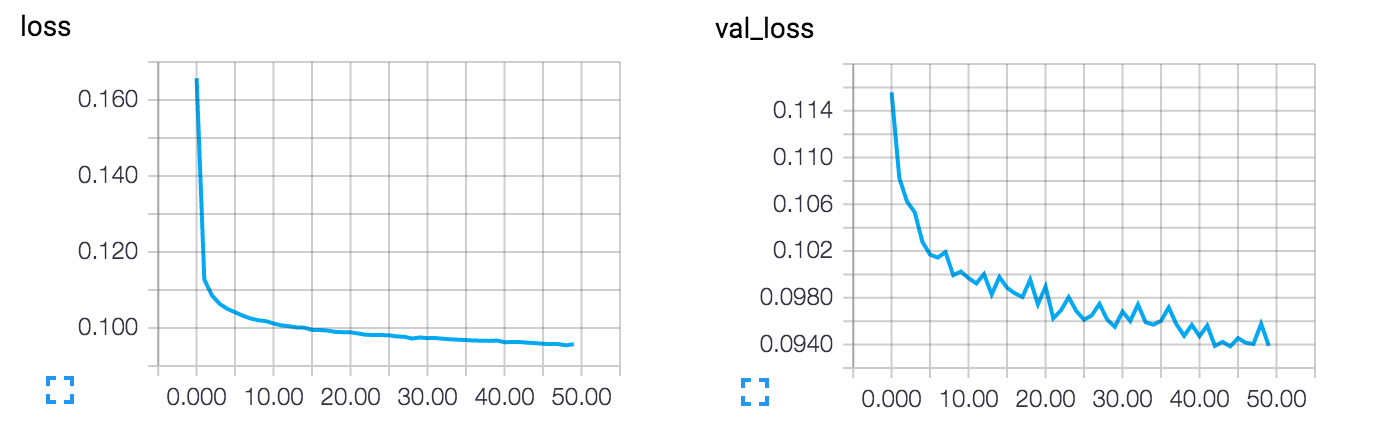
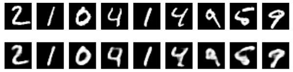
The model converges to a loss of 0.094, significantly better than our previous models (this is in large part due to the higher entropic capacity of the encoded representation, 128 dimensions vs. 32 previously). Let's take a look at the reconstructed digits:
decoded_imgs = autoencoder.predict(x_test)

n = 10
plt.figure(figsize=(20, 4))
for i in range(1, n + 1):
    # Display original
    ax = plt.subplot(2, n, i)
    plt.imshow(x_test[i].reshape(28, 28))
    plt.gray()
    ax.get_xaxis().set_visible(False)
    ax.get_yaxis().set_visible(False)

    # Display reconstruction
    ax = plt.subplot(2, n, i + n)
    plt.imshow(decoded_imgs[i].reshape(28, 28))
    plt.gray()
    ax.get_xaxis().set_visible(False)
    ax.get_yaxis().set_visible(False)
plt.show()
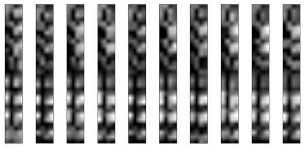
We can also have a look at the 128-dimensional encoded representations. These representations are 8x4x4, so we reshape them to 4x32 in order to be able to display them as grayscale images.
encoder = keras.Model(input_img, encoded)
encoded_imgs = encoder.predict(x_test)

n = 10
plt.figure(figsize=(20, 8))
for i in range(1, n + 1):
    ax = plt.subplot(1, n, i)
    plt.imshow(encoded_imgs[i].reshape((4, 4 * 8)).T)
    plt.gray()
    ax.get_xaxis().set_visible(False)
    ax.get_yaxis().set_visible(False)
plt.show()
Application to image denoising
Let's put our convolutional autoencoder to work on an image denoising problem. It's simple: we will train the autoencoder to map noisy digits images to clean digits images.
Here's how we will generate synthetic noisy digits: we just apply a gaussian noise matrix and clip the images between 0 and 1.
from keras.datasets import mnist
import numpy as np

(x_train, _), (x_test, _) = mnist.load_data()

x_train = x_train.astype('float32') / 255.
x_test = x_test.astype('float32') / 255.
x_train = np.reshape(x_train, (len(x_train), 28, 28, 1))
x_test = np.reshape(x_test, (len(x_test), 28, 28, 1))

noise_factor = 0.5
x_train_noisy = x_train + noise_factor * np.random.normal(loc=0.0, scale=1.0, size=x_train.shape)
x_test_noisy = x_test + noise_factor * np.random.normal(loc=0.0, scale=1.0, size=x_test.shape)

x_train_noisy = np.clip(x_train_noisy, 0., 1.)
x_test_noisy = np.clip(x_test_noisy, 0., 1.)
Here's what the noisy digits look like:
n = 10
plt.figure(figsize=(20, 2))
for i in range(1, n + 1):
    ax = plt.subplot(1, n, i)
    plt.imshow(x_test_noisy[i].reshape(28, 28))
    plt.gray()
    ax.get_xaxis().set_visible(False)
    ax.get_yaxis().set_visible(False)
plt.show()

If you squint you can still recognize them, but barely. Can our autoencoder learn to recover the original digits? Let's find out.
Compared to the previous convolutional autoencoder, in order to improve the quality of the reconstructed, we'll use a slightly different model with more filters per layer:
input_img = keras.Input(shape=(28, 28, 1))

x = layers.Conv2D(32, (3, 3), activation='relu', padding='same')(input_img)
x = layers.MaxPooling2D((2, 2), padding='same')(x)
x = layers.Conv2D(32, (3, 3), activation='relu', padding='same')(x)
encoded = layers.MaxPooling2D((2, 2), padding='same')(x)

# At this point the representation is (7, 7, 32)

x = layers.Conv2D(32, (3, 3), activation='relu', padding='same')(encoded)
x = layers.UpSampling2D((2, 2))(x)
x = layers.Conv2D(32, (3, 3), activation='relu', padding='same')(x)
x = layers.UpSampling2D((2, 2))(x)
decoded = layers.Conv2D(1, (3, 3), activation='sigmoid', padding='same')(x)

autoencoder = keras.Model(input_img, decoded)
autoencoder.compile(optimizer='adam', loss='binary_crossentropy')
Let's train it for 100 epochs:
autoencoder.fit(x_train_noisy, x_train,
                epochs=100,
                batch_size=128,
                shuffle=True,
                validation_data=(x_test_noisy, x_test),
                callbacks=[TensorBoard(log_dir='/tmp/tb', histogram_freq=0, write_graph=False)])
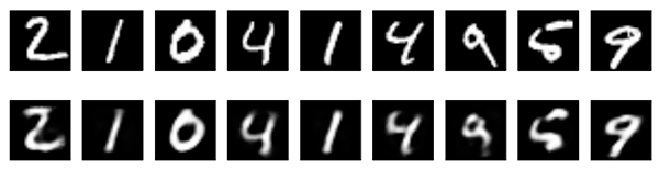
Now let's take a look at the results. Top, the noisy digits fed to the network, and bottom, the digits are reconstructed by the network.
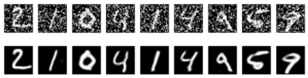
It seems to work pretty well. If you scale this process to a bigger convnet, you can start building document denoising or audio denoising models. Kaggle has an interesting dataset to get you started.
Sequence-to-sequence autoencoder
If you inputs are sequences, rather than vectors or 2D images, then you may want to use as encoder and decoder a type of model that can capture temporal structure, such as a LSTM. To build a LSTM-based autoencoder, first use a LSTM encoder to turn your input sequences into a single vector that contains information about the entire sequence, then repeat this vector n times (where n is the number of timesteps in the output sequence), and run a LSTM decoder to turn this constant sequence into the target sequence.
We won't be demonstrating that one on any specific dataset. We will just put a code example here for future reference for the reader!
timesteps = ...  # Length of your sequences
input_dim = ...
latent_dim = ...

inputs = keras.Input(shape=(timesteps, input_dim))
encoded = layers.LSTM(latent_dim)(inputs)

decoded = layers.RepeatVector(timesteps)(encoded)
decoded = layers.LSTM(input_dim, return_sequences=True)(decoded)

sequence_autoencoder = keras.Model(inputs, decoded)
encoder = keras.Model(inputs, encoded)
Variational autoencoder (VAE)
Variational autoencoders are a slightly more modern and interesting take on autoencoding.
What is a variational autoencoder, you ask? It's a type of autoencoder with added constraints on the encoded representations being learned. More precisely, it is an autoencoder that learns a latent variable model for its input data. So instead of letting your neural network learn an arbitrary function, you are learning the parameters of a probability distribution modeling your data. If you sample points from this distribution, you can generate new input data samples: a VAE is a "generative model".
How does a variational autoencoder work?
First, an encoder network turns the input samples x into two parameters in a latent space, which we will note z_mean and z_log_sigma. Then, we randomly sample similar points z from the latent normal distribution that is assumed to generate the data, via z = z_mean + exp(z_log_sigma) * epsilon, where epsilon is a random normal tensor. Finally, a decoder network maps these latent space points back to the original input data.
The parameters of the model are trained via two loss functions: a reconstruction loss forcing the decoded samples to match the initial inputs (just like in our previous autoencoders), and the KL divergence between the learned latent distribution and the prior distribution, acting as a regularization term. You could actually get rid of this latter term entirely, although it does help in learning well-formed latent spaces and reducing overfitting to the training data.
Because a VAE is a more complex example, we have made the code available on Github as a standalone script. Here we will review step by step how the model is created.
First, here's our encoder network, mapping inputs to our latent distribution parameters:
original_dim = 28 * 28
intermediate_dim = 64
latent_dim = 2

inputs = keras.Input(shape=(original_dim,))
h = layers.Dense(intermediate_dim, activation='relu')(inputs)
z_mean = layers.Dense(latent_dim)(h)
z_log_sigma = layers.Dense(latent_dim)(h)
We can use these parameters to sample new similar points from the latent space:
from keras import backend as K

def sampling(args):
    z_mean, z_log_sigma = args
    epsilon = K.random_normal(shape=(K.shape(z_mean)[0], latent_dim),
                              mean=0., stddev=0.1)
    return z_mean + K.exp(z_log_sigma) * epsilon

z = layers.Lambda(sampling)([z_mean, z_log_sigma])
Finally, we can map these sampled latent points back to reconstructed inputs:
# Create encoder
encoder = keras.Model(inputs, [z_mean, z_log_sigma, z], name='encoder')

# Create decoder
latent_inputs = keras.Input(shape=(latent_dim,), name='z_sampling')
x = layers.Dense(intermediate_dim, activation='relu')(latent_inputs)
outputs = layers.Dense(original_dim, activation='sigmoid')(x)
decoder = keras.Model(latent_inputs, outputs, name='decoder')

# instantiate VAE model
outputs = decoder(encoder(inputs)[2])
vae = keras.Model(inputs, outputs, name='vae_mlp')
What we've done so far allows us to instantiate 3 models:
- an end-to-end autoencoder mapping inputs to reconstructions
- an encoder mapping inputs to the latent space
- a generator that can take points on the latent space and will output the corresponding reconstructed samples.
We train the model using the end-to-end model, with a custom loss function: the sum of a reconstruction term, and the KL divergence regularization term.
reconstruction_loss = keras.losses.binary_crossentropy(inputs, outputs)
reconstruction_loss *= original_dim
kl_loss = 1 + z_log_sigma - K.square(z_mean) - K.exp(z_log_sigma)
kl_loss = K.sum(kl_loss, axis=-1)
kl_loss *= -0.5
vae_loss = K.mean(reconstruction_loss + kl_loss)
vae.add_loss(vae_loss)
vae.compile(optimizer='adam')
We train our VAE on MNIST digits:
(x_train, y_train), (x_test, y_test) = mnist.load_data()

x_train = x_train.astype('float32') / 255.
x_test = x_test.astype('float32') / 255.
x_train = x_train.reshape((len(x_train), np.prod(x_train.shape[1:])))
x_test = x_test.reshape((len(x_test), np.prod(x_test.shape[1:])))

vae.fit(x_train, x_train,
        epochs=100,
        batch_size=32,
        validation_data=(x_test, x_test))
Because our latent space is two-dimensional, there are a few cool visualizations that can be done at this point. One is to look at the neighborhoods of different classes on the latent 2D plane:
x_test_encoded = encoder.predict(x_test, batch_size=batch_size)
plt.figure(figsize=(6, 6))
plt.scatter(x_test_encoded[:, 0], x_test_encoded[:, 1], c=y_test)
plt.colorbar()
plt.show()
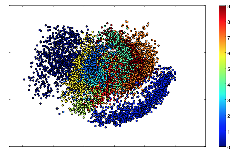
Each of these colored clusters is a type of digit. Close clusters are digits that are structurally similar (i.e. digits that share information in the latent space).
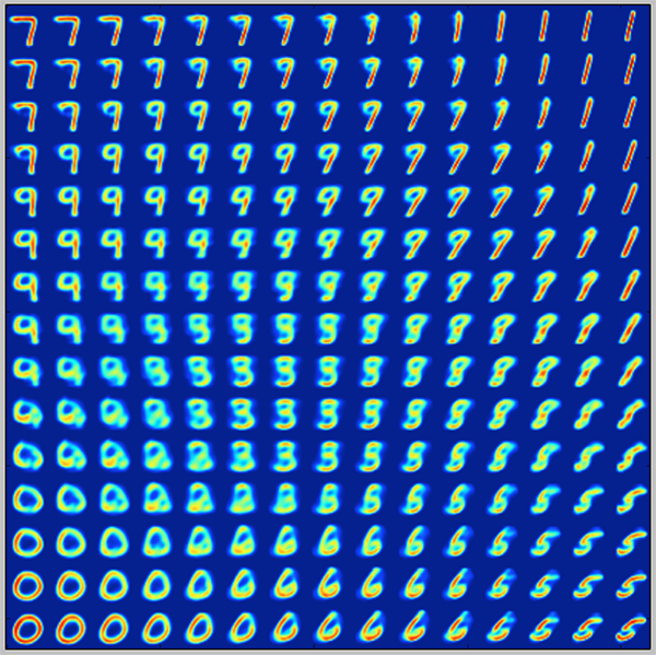
Because the VAE is a generative model, we can also use it to generate new digits! Here we will scan the latent plane, sampling latent points at regular intervals, and generating the corresponding digit for each of these points. This gives us a visualization of the latent manifold that "generates" the MNIST digits.
# Display a 2D manifold of the digits
n = 15  # figure with 15x15 digits
digit_size = 28
figure = np.zeros((digit_size * n, digit_size * n))
# We will sample n points within [-15, 15] standard deviations
grid_x = np.linspace(-15, 15, n)
grid_y = np.linspace(-15, 15, n)

for i, yi in enumerate(grid_x):
    for j, xi in enumerate(grid_y):
        z_sample = np.array([[xi, yi]])
        x_decoded = decoder.predict(z_sample)
        digit = x_decoded[0].reshape(digit_size, digit_size)
        figure[i * digit_size: (i + 1) * digit_size,
               j * digit_size: (j + 1) * digit_size] = digit

plt.figure(figsize=(10, 10))
plt.imshow(figure)
plt.show()
That's it! If you have suggestions for more topics to be covered in this post (or in future posts), you can contact me on Twitter at @fchollet.
References
[1] Why does unsupervised pre-training help deep learning?
[2] Batch normalization: Accelerating deep network training by reducing internal covariate shift.